A note: You might want to scroll down, directly to Applying the NetLogo model to avoid my long winded setup and context)
Getting Stuck in a Rut:
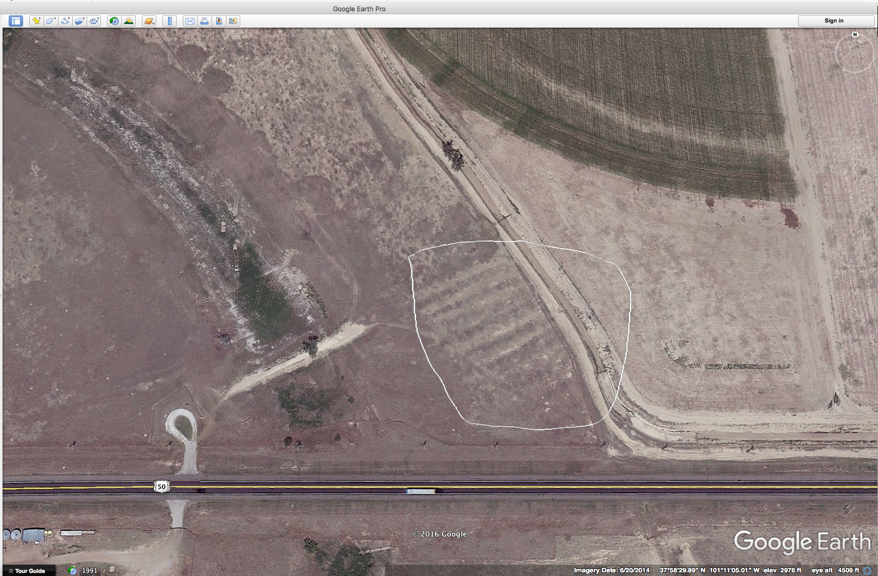
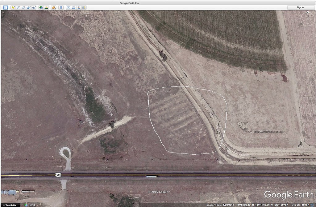
I grew up about 1 mile from the Santa Fe Trail which cuts diagonally across Kansas on its way from Independence, Mo. to Santa Fe, New Mexico. And I have lived most of my adult life close to the trail. Not everyone is familiar with this historical trail so here’s a quote from the Santa Fe Trail Association’s website that might put things into context: “In 1821, the Santa Fe Trail became America’s first great international commercial highway, and for nearly sixty years thereafter was one of the nation’s great routes of adventure and western expansion. ” For folks growing up on the plains, the trails are kind of a big deal. For instance, along U.S. highway 400/50 in western Kansas you can pull over, park and walk in the ruts of the trail that still exist. Here’s a Google Earth screen shot of the ruts trending to the SW. I have put a white polygon around the ruts. Amazing, isn’t it?
Well, the short answer is that I think we, the teacher community, are particularly at risk of getting “stuck in a rut.” Like the folks on the Santa Fe trail we are often looking for direct, point to point solutions for many of the challenges that surface in a classroom of students who all have different skills and backgrounds. Take for example, “The Scientific Method”. Here, was a simplification designed originally by Paul Brandwein to make science as a verb more accessible to both teachers and students. Of course it was a simplification and of course, if Paul were still here, he’d be appalled at how one-dimensional this model has become. We do that in science education–we make ruts—deep ruts. Another example, that strikes close to home is the former AP Biology Lab manual–a series of labs that became known as the “Dirty Dozen” that folks felt they had to follow to the letter while almost always neglecting or ignoring the suggestions at the end of each laboratory for further, deeper investigations–another deep rut.
As many of you know, I’ve spent the last 9 years helping to prepare math and science teachers in the UKanTeach program. In this program we introduce the students to the 5E lesson plan model to help them prepare effective (and efficient) lessons that are steeped in inquiry. The design works fairly well and really serves as a great scaffold to build an effective lesson or series of lessons around. Those of you familiar with the model may recognized that one could deconstruct these series of posts down into the 5E’s. Engage, Explore, Explain, Extend, and Evaluate. But, to avoid our basic nature of creating a rut to fall into, I’ve purposely left out any explicit designation, notation or label consistent with the 5E’s. Part of that is because, I think you can see that some folk’s Extension activity might be another’s Evaluation activity. It depends on the context in my opinion. Perhaps more importantly, is that I don’t want to suggest that teaching quantitative skills is a linear process. Following linear paths, creates ruts. Instead, I hope I presented a multitude of paths or at least suggested that this lab is a very rich resource that opens all sorts of options you might consider. It is up to you, the trail boss to decide how you plan to guide your class over the quantitative skills landscape and hopefully, you’ll find it rewarding to the point of taking quantitative skill instruction beyond what I’ve suggested here.
With that said, I am going to present material here that might fit more appropriately in the Extend or Evaluate phase of a 5-E lesson. I see a couple of paths forward. One takes the quantitative and content level skills learned in this exploration and applies them in an another laboratory investigation and the other takes those same skills but applies them in model-based environment. Doubtlessly there are many other paths forward for you to discover but let’s focus on these for now.
A model environment that probes deeper into thinking about enzyme reaction kinetics:
But first some more history/ reminiscing.
In the 1980’s when personal computers first arrived on the educational scene one of the first applications were programs that provided simulations of biological phenomena. I even wrote one that students could use to generate inheritance data with simulated fruit fly crosses. I was pretty proud of it to the point that I actually marketed it for awhile. Students had to choose their parent flies with unknown genotypes from primitive graphic images that provided phenotype information. Once a cross was chosen, then the program would randomly according to the inheritance pattern generate about 48 fly images that represented the phenotypes possible. The student had to infer genotypes from phenotypes. However, when I wrote this program I created an option where the student could pick and choose the inheritance pattern to investigate. So the program only simulated data to confirm a given inheritance pattern. The data was realistic since it used a random function to generate gametes but it could have promoted more inquiry and scientific thinking. I found this out when I cam across the Genetics Construction Kit (GCK) a piece of software written by John Calley and John Jungck. This program lacked the graphics that mine had but it promoted inquiry much, much better. Students didn’t start by choosing an inheritance patter. Instead, they received a sample “vial” of flies with a number of different traits expressed. They had to choose different flies, different traits and such and then design crosses, form hypotheses, look for data to support those hypotheses and go to work. It was a revelation. Even better to my way of thinking it “modeled” almost every type of inheritance you could study in those days. Even more better—the program didn’t tell the student if they were right or wrong. The student (and the teacher) had to look at the various crossing data to determine if the data supported their hypothesis. This was an excellent educational tool to teach genetics. If you and your students could meet the challenge I guarantee that the learning was deep. (Collins, Angelo, and James H. Stewart. “The knowledge structure of Mendelian genetics.” The American Biology Teacher 51.3 (1989): 143-149.) If you don’t have access to JSTOR you can find another paper by Angelo Collins on the GCK here: Collins, Angelo. “Problem-Solving Rules for Genetics.” (1986). I promoted the GCK heavily throughout the late 80’s and 90’s. I still think it is an inspired piece of software. The problem was that little bit about not providing answers. Few of my teaching colleagues were comfortable with that. I’d round up computers or a computer lab for a presentation or professional development. Everything would be going smoothly. There would be lots of ooh’s and aw’s as we worked through the introductory level and then everything would so south when the teachers would find out that even they couldn’t find out what the “real” answer was. Over and over, I’d ask; “Who tells a research scientist when they are right?” but it wasn’t enough. Teachers, then were not as comfortable without having the “real” answer in their back pocket. I think that has changed now at least to some degree.
The software world has changed as well. GCK went on to inspire Bioquest. From their website: “BioQUEST software modules and five other modules associated with existing computer software, all based on a unified underlying educational philosophy. This philosophy became known, in short, as BioQUEST’s 3P’s of investigative biology – problem posing, problem solving, and persuasion.” Another early “best practice” educational application of computer technology was the software LOGO from Seymour Papert’s lab. LOGO was agent based programming specifically targeted to students early in their educational trajectory. My own children learned to program their turtles. As the web developed and other software environments developed LOGO was adapted into NETLOGO.
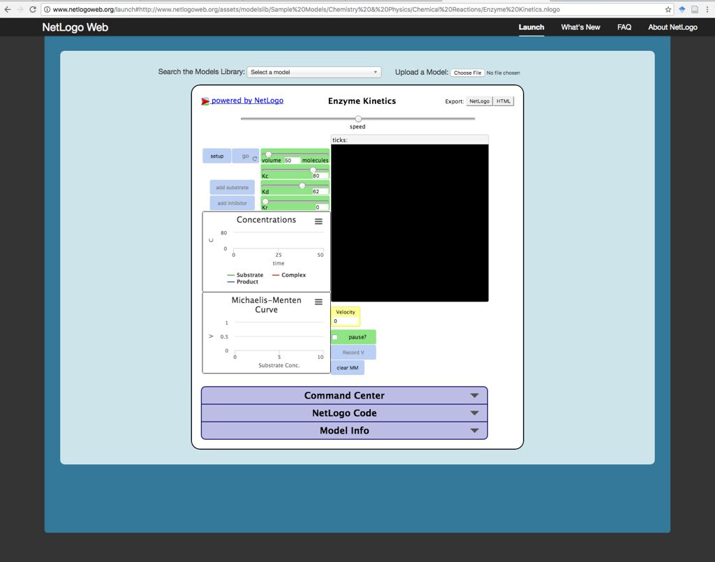
Netlogo (Wilensky, U. (1999). NetLogo. http://ccl.
Applying the NetLogo Model:
The NetLogo model is built on the same conceptual model for enzyme kinetics that we have explored before:
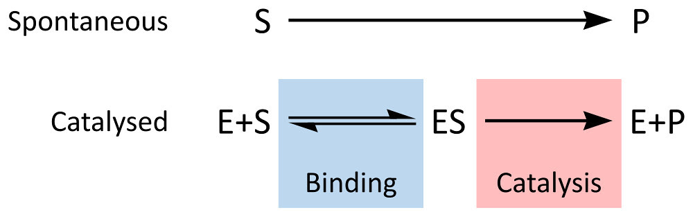
By Thomas Shafee (Own work) [CC BY 4.0 (http://creativecommons.org/li
Constant 1: The rate of formation of the ES complex.
Constant 2: The rate of dissociation of the ES complex back into E and S
Constant 3: The rate of catalysis of the ES complex into E and P
You explore the model by changing these constants or changing the substrate concentration. Changing the constants, changes the properties of the enzyme.
http://ccl.
I’ve put together a short video of that introduces how one might work with this model to create data similar to the data from the original wet lab. You can find it here:
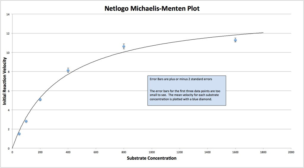
Here’s a M-M curve that I generated by changing the values of the constants and then seeing how those properties determined Enzyme rates/velocities at differing substrate concentrations.
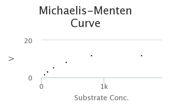
In this curve I collected, 8 samples for each substrate concentration.
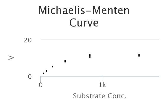
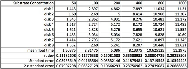
Here’s the data, generated by the model. Looks a lot like the wet-lab data, doesn’t it?
And here is a curve fit to the Michaelis-Menten equation. Note that the data from the NetLogo model has to be fitted to the idealized curve.
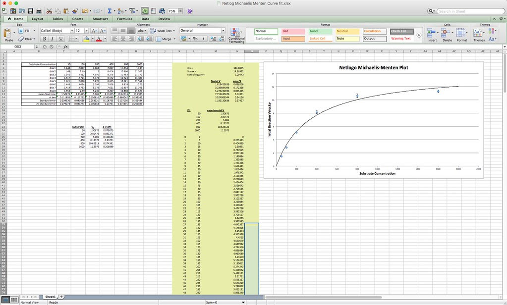
Note that the data from the NetLogo model has to be fitted to the idealized curve.
The thing is that I could go back into the Netlogo model and explore questions like, what happens if I lower the constant that describes the rate of Enzyme-Substrate formation relative to the constant that describes the dissociation of that complex? Several questions come to mind.
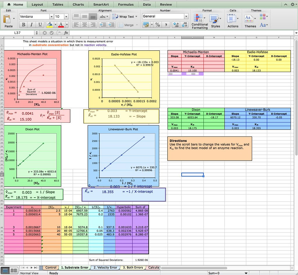
Of course you don’t have to explore Netlogo as an extension or evaluation activity. You could have your students explore this spreadsheet from the Bioquest Esteem project:
Michaelis-Menten Enzyme Kinetics
Or if you are really ambitious you could have your students develop their own spreadsheet model like the one described in this paper from Bruist in the Journal of ChemEd.
Bruist, M.F. (1998). Use of a Spreadsheet To Simulate Enzyme Kinetics. Journal of Chemical Education, 75(3), 372. http://biochemlab.org/wp-cont
Or you could have your students explore the AP Biology Community’s own Jon Darkow Stella-based model for lactase enzyme activity: https://sites.google.com/site
Practice, Practice, Practice (Curve fitting in the Photosynthesis Floating Leaf Disk lab)
To master any skill takes lots of practice–something we don’t provide enough of in academic classes. We do in the performance and fine art classes but not so much in academics. The excuse as to why not usually gets back to the extreme time limitation we face in the biology classroom. Still with the right selection of lab topics skill practice is not only possible but highly productive. For instance in this case, it turns out that the procedure, the data created, the data analysis, the curve fitting (to the same mathematical model) are all skill that can be applied to the Floating Leaf Disk lab, if the students explore how the intensity of light affects the rate of photosynthesis.
In 2015, Camden Burton and I presented some sample data sets from the Floating Leaf Disk lab at NABT. Later I shared those in a series of posts on the AP Biology Community forum where a lively discussion on data analysis ensued. If you are a member of the forum you can find the discussion here.
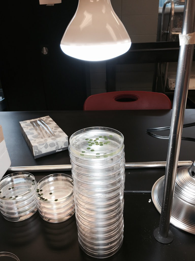
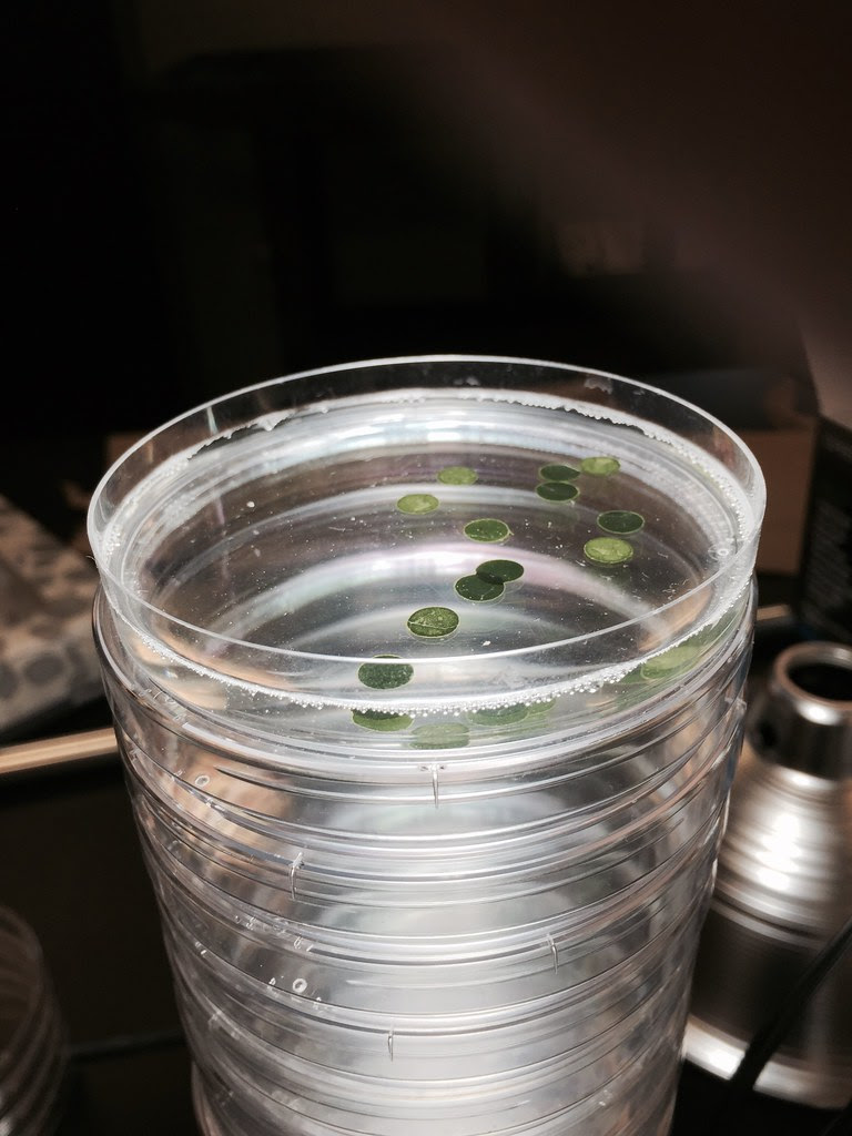
One of the more problematic data sets we shared was data from a photoresponse curve experiment that explore how light intensity affects the rate of photosynthesis. Here’s a photo of how light intensity was varied by varying the height of the stack of petri dishes.
Here’s the raw data for this lab using the lap timer on a smart phone:

The first step working with this data is to convert the lap times into cumulative times along with generating the descriptive stats.
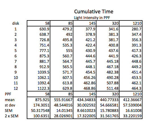
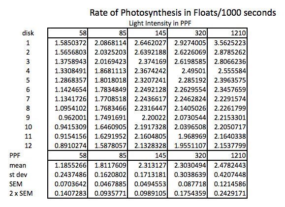
Because the how fast a disk rises with this technique is inversely proportional to the actual rate of photosynthesis we need to convert this time into a rate by taking the inverse or the reciprocal. And since this turns out to be a small decimal number with the units of float/sec, I’ve modified it by multiplying by 1000 seconds to get a rate unit of float per 1000 seconds. The descriptive stats are converted/transformed in the same way. This process of data transformation is not emphasized enough at the high school level in my opinion.
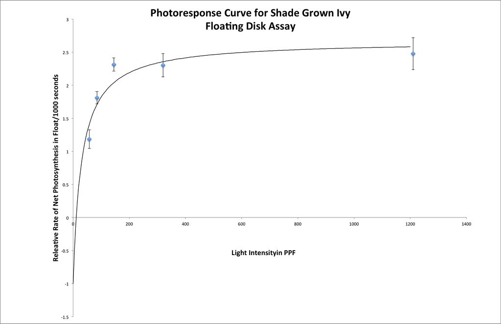
Graphing the means in this data table along with plus or minus 2 SEM error bars creates a graph something like this:
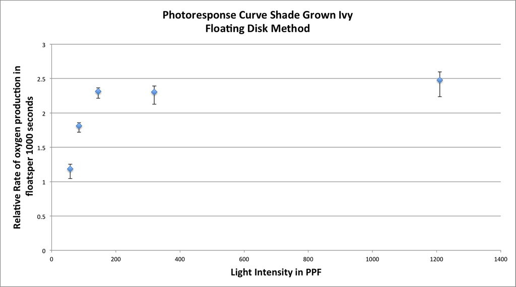
Which in my mind is a curve waiting to be fitted. If you google something like “Photosynthesis Irradiance Curve” you’ll find a number of resources applicable to this experiment and guess what? You’ll find that folks have been using the Michaelis-Menten equation to model the curve fitting.
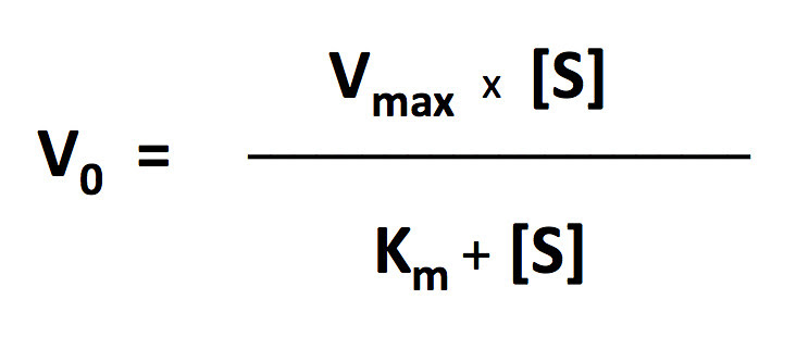
I’ll let you explore the resources but here is the fit based on the Michaelis-Menten equation. There is a modification to the Michaelis-Menten expression that we have to do for this particular lab. Since this procedure actually is measuring the accumulation of oxygen as a product and some of the oxygen is being consumed at the same time for cellular respiration, we are actually measuring the net rate of photosynthesis. To account for the oxygen consumed in respiration we need to add an additional term to the Michaelis-Menten equation. 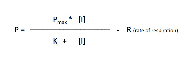
I’ve changed the variables but the form of the equation is the same. In the curve fitting that I have done, I have manually changed the value of R and let the solver vary Pmax and KI.
The fit for this set of data is not as good as we got for the catalase lab but it is not bad.
Interestingly, you can get a “good” fit to an exponential function as well–maybe even a better fit. But, that is part of model fitting. There is many biological reasons to consider that Michelis-Menten provides a model for photosynthesis but I can’t think of one for an exponential fit. There are many ways to continue to modify the Michaelis Menten application to Photosynthesis Irradiance curves and you can find several with a bit of google searching.
Here’s one fit I managed in excel using the same techniques that we used earlier.
Here is a Desmos version you or your students can play with.
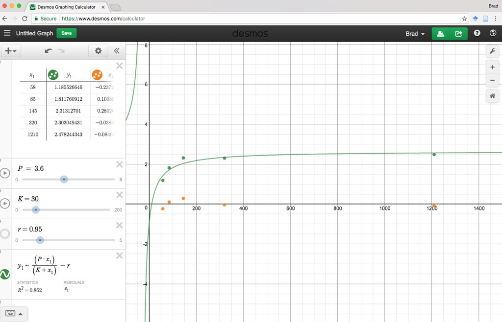
https://www.desmos.com/calcula
I think it is time to wrap this series of long winded posts up. I hope, if you’ve read this far, that you have found some ideas to try in your class and I hope that despite the deep dive that an idea of how an increased emphasis on quantitative skills can also lead to an increase understanding of the content–at least it does for me. Finally, I hope you and your students have a good time exploring data analysis—it really does feel good when the data works out like you think it should. 😉