I apologize for the length of these posts but I had a couple of goals in mind when I decided to “rewrite” these posts on modeling populations that had been lost from the old NABT BioBlog: 1. To help biology educators develop their own confidence to take on computer-based modeling in their classroom and 2. To give an accounting of the types of thinking that went on in my mind and in my students’ minds as we explored this area. I think the previous two posts on this topic address these goals. (https://www.bradwilliamson.net/a-wee-bit-of-math-geekery/ and https://www.bradwilliamson.net/using-spreadsheets-to-build-simple-models-of-population-growth/) This post is a little extra gravy on top. I suspect that most biology educators will not see a need to explore at this depth but maybe I’m wrong–let’s see how it goes. Like the other two posts, you can follow along with a google sheet at: https://docs.google.com/spreadsheets/d/11cMOAnw9qO1gzuY3-Zl47QtQP72H6Bq0cLDKPuj_thc/edit?usp=sharing
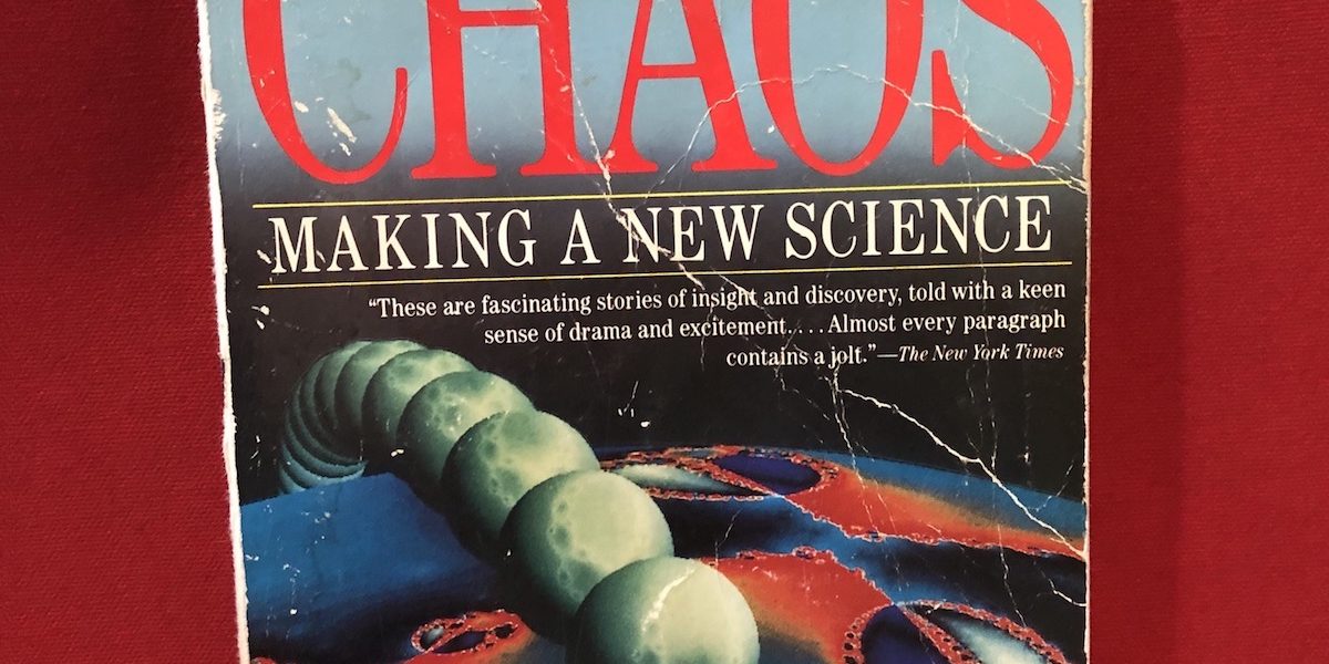
Sometimes you make elaborate plans and preparations for class and sometimes things just happen. In the late 1980s, James Gleick wrote a book titled: Chaos Making a New Science.
I was fascinated by this book and was actually looking for an opportunity to explore some of its concepts with my students. I had the software that accompanied the book and shared quite a bit of fractal geometry, the game of life, and Mandelbrot sets with my students in an informal way, searching for what was relevant and what might make a difference in their future. Up to this point, I had not found topics that were quite accessible and interesting enough to devote formal class time to, although the students loved to play with the Mandelbrot sets to see how far down they could explore self-similarity. But once the students figured out the logistic expression I knew we had to do more.
An essential part of the modeling process that is often overlooked is testing or even stressing your model to see how well it holds up, to define with precision what it is telling you, to help you define its limitations, to establish your confidence in it and to evaluate how well it works. Most folks seem to want to get right to the predictions that can come from a model but I rather enjoy the tweaking part. I knew that our logistic model had some surprises in store for the students once they began testing how the parameters interacted. You see, chapter 3 from Gleick’s book was on Robert May’s mathematical modeling work. May had discovered an entirely new set of outcomes to consider when modeling with difference equations (like this discrete model)–an area of chaos, instability, and unpredictability. Interestingly, he had discovered these surprises by playing with the logistic model with one of the first programmable calculators in the 1970s so I knew we could do the same with our computer-based spreadsheet model but I had not really tried it but now was my chance–my students would recreate some of Robert May’s discoveries. Gleick finished up chapter three with this quote from May’s 1976 paper, Simple mathematical models with very complicated dynamics,
“Not only in research, but also in the everyday world of politics and economics, we would all be better off if more people realized that simple nonlinear systems do not necessarily possess simple dynamical properties.”
Robert May died last month, as I write this. If you haven’t included his work in your Biology class–do consider doing so–especially in light of the Covid-19 pandemic. He was a leading epidemiologist who helped develop the R0 concept. From the New York Times: https://www.nytimes.com/2020/05/11/science/robert-may-dead.html
Heady stuff–doing what you should do but getting some icing on the cake: Test the model, and then finding this wild new world of chaos or non-linear dynamics. So we started to tweak the parameters of the model.
We had a bit of a discussion about just what does it mean to “test” your model. I tried to direct the instruction to the idea that they systematically (with a plan) change their parameters incrementally, one small step at a time, and try to discern any patterns that they see. Doing so would likewise require keeping a record of the changes while recording their thinking. They had their lab notebooks for that. So they set to work. The quickly discovered that the K parameter didn’t change much in the nature of the result–only effecting how long it took to get to carrying capacity. But it did not take them long to see that changing the r parameter made a change–sometimes a big change. For this reason, we focused on the r term (and this likewise is where the Robert May work focused as well.)
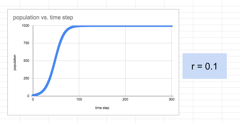
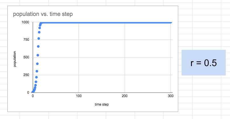
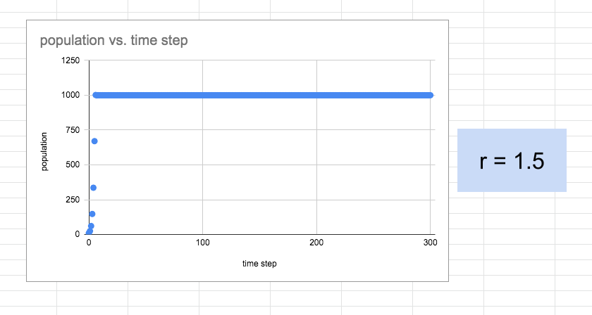
The students, all, quickly determined that the higher the r-value, the steeper the S-curve. Pretty much all the students also stopped when they got close to r = 1 which I guess they thought was some sort of limit. I had to gently suggest they move beyond r = 1 but did so after re-examining just what the r-value represented in the model. Essentially, a value of r = 1 meant that the increase in each time interval was equivalent to a 100% increase. Hmmmmm. Note that it only takes 5 times steps to reach a carrying capacity of 1000 with the model set to r = 1.5
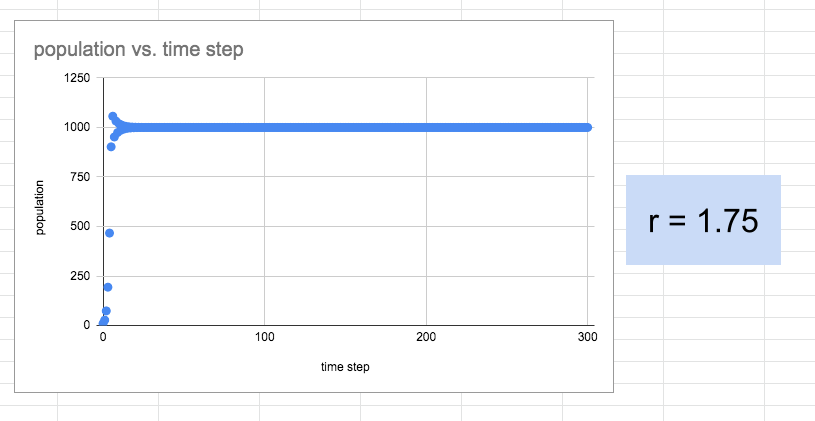
After all this “exploration” and recording their observations in their notebooks, they are beginning to feel they have a handle on the model. At this point, the students are actually starting to get a bit bored and are thinking that this is just plain common sense (of course, not remembering where they were a couple of days before.) Usually, I have to say something along the line of “Well, let’s keep this up until an r = at least 3 or 4.” Naturally, there are some that protest but go along with the suggestion. And then……boom, this happens.
Their interest is perking up.
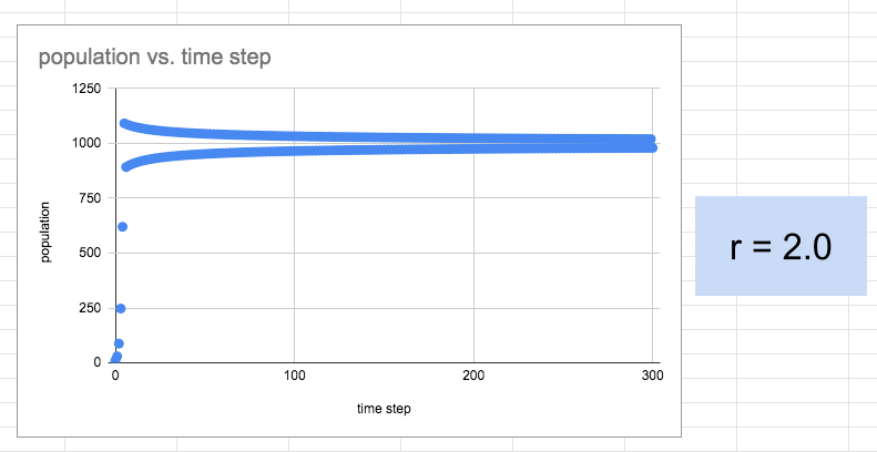
Now I’ve got their attention again. “Hey, what’s going on?” “How does it go above 1000?” We have to revisit the nature of the computational model. Difference equations, growth rates more than 150% in a single time interval, overshoots, undershoots–all are part of the discussion. But still, look at those “stable” outcomes–“There seems to be two carrying capacities.” “Does that even make sense in the real world?” It doesn’t take much encouragement for them to try changing things a bit more.
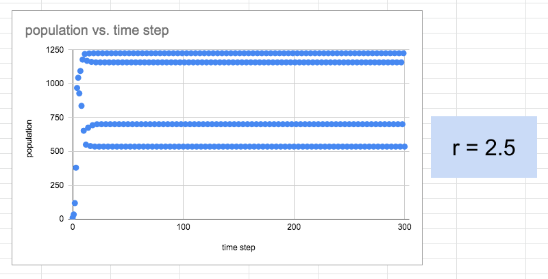
There is some beauty going on here. Very cool pattern, with four “stable” carrying capacities with two above the original 1000. I wonder if we can get to 8 or 16? Student engagement/surprise is pretty high at this point although I think they have forgotten that we were trying to model population growth.
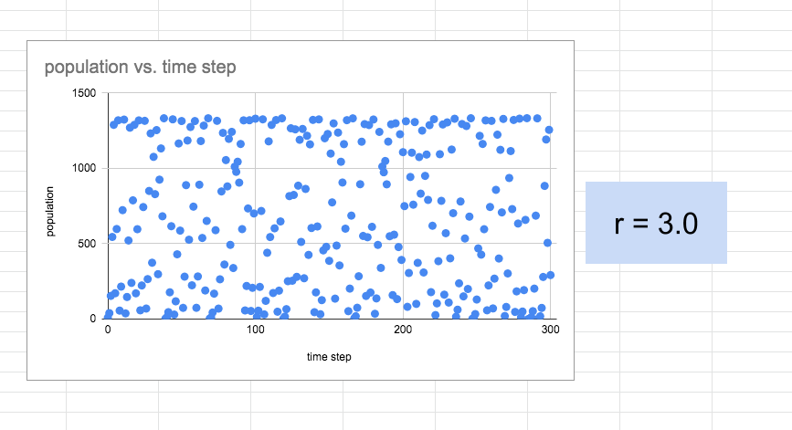
“What happened?” “Did I break it?” With my college students who had a calculus background, we’d talk at this point about the differences between discrete models and continuous/instantaneous models and the benefits of each. After which I would bring Robert May into the discussion. For my high school students, I went right to the discussion about Rober May and his work in the 1970s with this very equation. We’d wrap up with a discussion on why this might be important and a revisit to our original intent.
Robert May used a slightly different version of this equation but you can get a feel for it and how important it is for scientific models in general from this great video from Veritasium: Veritasium on chaos: https://www.youtube.com/watch?v=ovJcsL7vyrk Note that he is taking us to some other areas that are possible with a bit more math so his results and “r” values look a little different. Note there is no K term.
I first wrote about this activity in the, now defunct NABT BioBlog. Since then a number of folks have also discovered spreadsheet population modeling along with the chaos extension. Here’s an example a one that is particularly well done along with a PowerPoint to help guide the student’s exploration in EXCEL or to help you the first time if you decide to try this with your students. https://serc.carleton.edu/sp/ssac_home/general/examples/19171.html Whether you work this activity from scratch, use Ben Steele’s work or just share Veratasiums video, I hope you give it a try.
Bibliography
Gleick, James. Chaos: Making a new science. Open Road Media, 2011.
May, R. Simple mathematical models with very complicated dynamics. Nature261, 459–467 (1976). https://doi.org/10.1038/261459a0