Computers and spreadsheets truly changed much of the way I taught biology, starting in the ’80s. Interestingly, spreadsheets were not on my radar early in the introduction of personal computers. Instead, I was sure that my students would be developing programming skills that would let us build models. (I may have been a bit “off” on that prediction.) It is hard to predict the effect of technology but there is no doubt the overall impact of computers in the classroom has been immense but I’d argue it is still far short of its potential.
In the mid-80’s I taught evening classes on computer applications for the local community college: word processors, spreadsheets, and others. I learned a lot about how challenging some find the “logic” of computer software design to be. Also, at this time I ended up in charge of our first computer lab at the small rural school where I taught. The application software was just making its appearance and was very costly. Hence, unbelievable, today, the sole focus of the computer lab was to teach programming. Only later, did we feature applications like word processors and spreadsheets. Funny how things change. At any rate, I did take the opportunity to take my biology classes down to the computer lab to use the word processing software to write their biology themed writing assignments. This turned out to be very successful and each quarter we had at least one significant writing assignment. However, I didn’t explore biology concepts using spreadsheets with students.
For me, an important milepost happened one summer while taking an NSF sponsored program on Yeast Genetics at Kansas State University. As part of the project, we each got a computer that had an early open-source spreadsheet program installed. At this workshop, I remember working with a theoretical physicist, Larry Weaver. One day, I played around with the idea of modeling a predator-prey model on the spreadsheet. In my classes, we had used a pencil and paper-based simulation of predator-prey cycles that involved beans, spoons, and paper sacks. The beans were rabbits, the spoons were coyotes and the sack was the environment. We had rules that defined how many rabbits a coyote had to catch in order to survive and/or reproduce and other rules about rabbit births. I simply interpreted the rules into a spreadsheet that I iterated and ended up creating classic Lotka-Volterra cycles. Larry was fascinated and exclaimed that had he had a tool like this back when he was in college he wouldn’t have needed calculus–he could just model it. He was, of course, exaggerating but not by much. His comment really resonated with me and I’ve worked ever since trying to leverage the power of the spreadsheet and computer to try and make complex, mathematical analysis accessible to all students. Why should the calculus students have all the fun?
In the late 80’s I moved to a suburban school district with lots of resources but I no longer had my own computer lab so I had to wait a couple of years before I could scrounge together enough computers for my classroom which I finally did in about 1992. Once the computers were in place, naturally I needed to start introducing computer-based models and the old BSCS Sparrow lab was the place I started.
(https://www.bradwilliamson.net/a-wee-bit-of-math-geekery/)
But this time, instead of pencil and paper, we built a spreadsheet table and used the spreadsheet to do our graphing. Even with taking time to teach the students, spreadsheet basics we had an exponential graph and a log graph in less than 30 minutes. This was a particularly easy spreadsheet model because the syntax was so simple and straightforward. There was no need for absolute referencing and the fill down function was a big hit. Here’s what it looked like but in Google sheets:
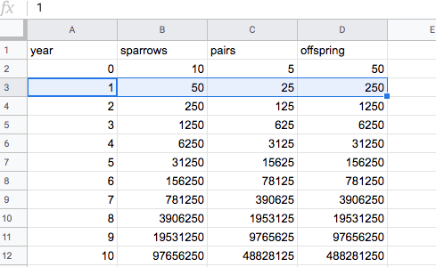
And with two graphs–one with the y-axis logged.
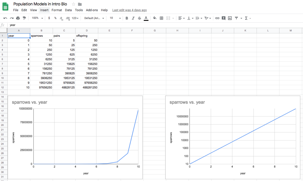
And a link to the actual spreadsheet, in case you want to make one, yourself:
https://docs.google.com/spreadsheets/d/11cMOAnw9qO1gzuY3-Zl47QtQP72H6Bq0cLDKPuj_thc/edit?usp=sharing
This exercise turned out to be dissatisfying in some ways. First of all, it went so fast I’m sure the students didn’t pick much up from the model building process–they focused too much on getting the details of the spreadsheet to work. They certainly, missed the “feel” for exponential growth because they didn’t have to scale their graph–again the computer did that for them. Nor did they develop as deep an understanding of logs compared to previous classes. In this particular application, I really thought that the computer created more of a pursuit of “the answer” instead of focusing on the question and how we get there. Not my kind of classroom experience. I was sorely tempted to simply chuck it and go back to pencil and paper but decided that perhaps this ease of making a computer-based model would serve to invite students into a deeper exploration of the modeling process and maybe—just maybe logistic growth models. I decided that as a class we needed to explore population modeling more deeply
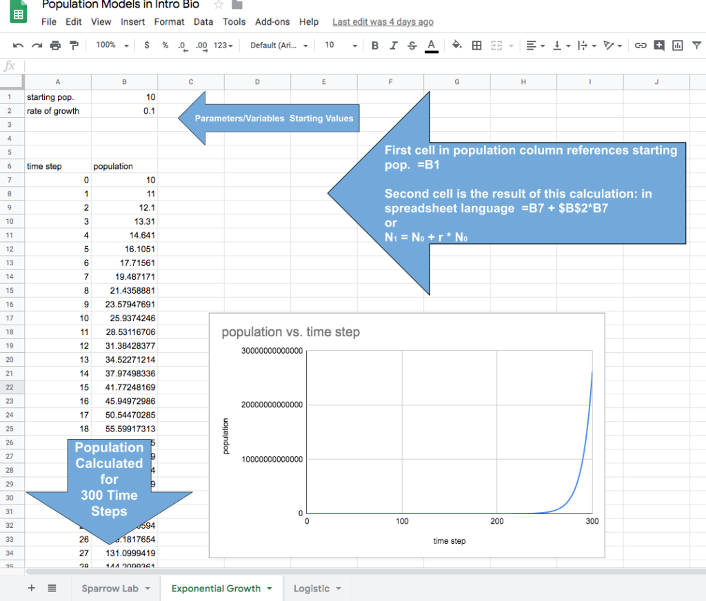
First, we revisited our sparrow population growth model and tried to distill it down into one or two variables and/or parameters. Through discussion, we came to the consensus to focus on time, population size and growth rate (or decline). Since we had already started using spreadsheets we simply added another sheet and got to work. Next, we defined our starting variables. Starting population size and growth rate. We documented our time in one column as steps from 0 to 300, again using the fill down procedure. We also created a column that recorded the population at each time step. I drew something like this on the board to guide their spreadsheet construction.
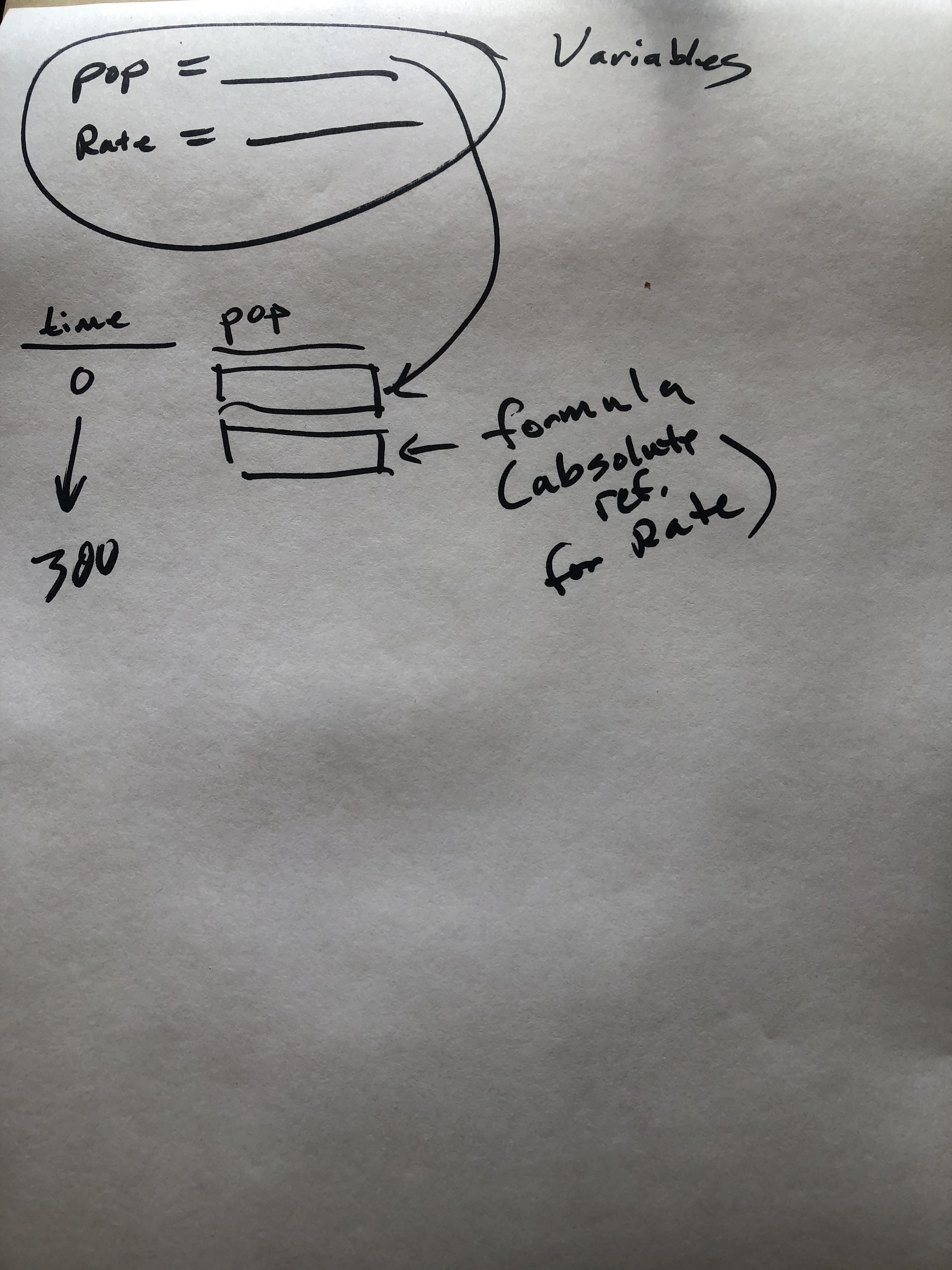
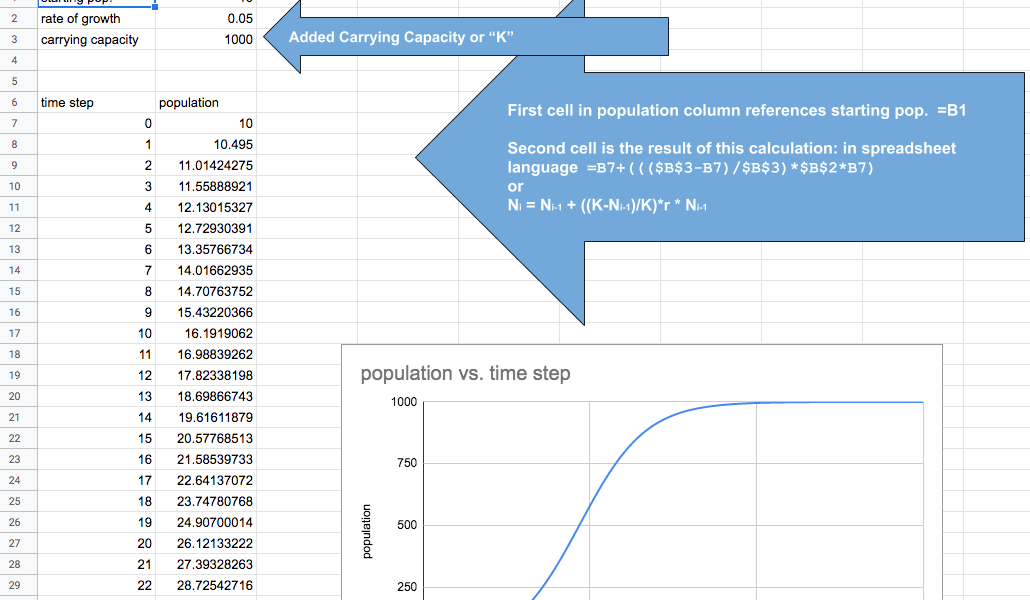
Now came the hard part. How do we make a formula that will take the original population, determine the change in the population and derive the new population for the next time step? With a little back and forth we came up with an equation that might work. Ni = Ni-1 + r* Ni-1 We had to learn a few spreadsheet skills in order to translate this equation into spreadsheet formulae–specifically we need to learn about fixed and absolute referencing. We wanted “r” to always remain the same but we wanted the N to change as the population grew or declined. Interpreting the formula into spreadsheetese generated the following:
=B7 + $B$2*B7
The “B7” for this cell is a relative cell address reference that will change incrementally as we copy the formula down. In the next cell down it will be “B8” and the next down after that it will be “B9” and so on. The “$’s” make “$B$2” an absolute cell address reference, which means that as the formula is copied this reference stays constant, always pointing to “B2” and the value for “r” that we enter there. (By the way, you can use the link above to this google sheet as well–it is the second tab.)
I honestly don’t remember how long it took to get to this point the first year I tried this. I know we hadn’t quite used up the hour, yet. I also know, that my years of teaching spreadsheets in computer classes paid off because I was able to help the students troubleshoot their spreadsheets since I’d seen most of the errors that are typically made. In later years, as my own skills working with spreadsheets and high school students improved, it would usually take about 30 minutes to get to this point in the modeling process.
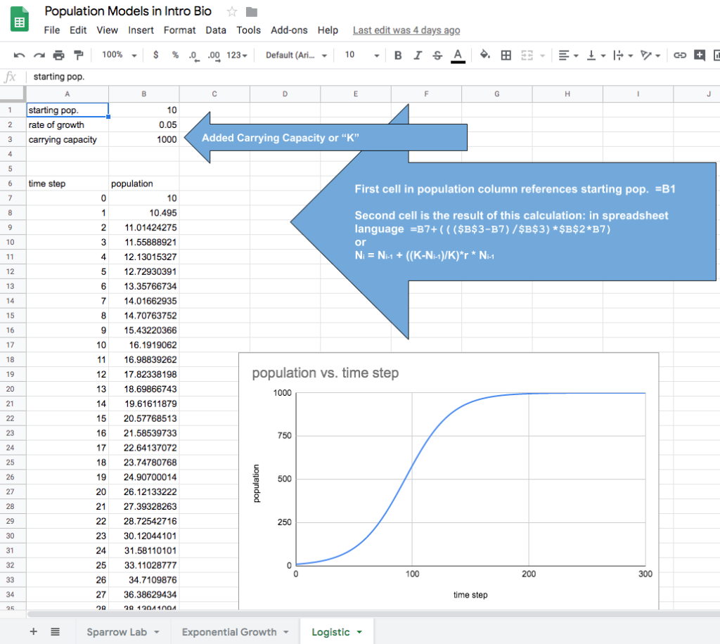
It was now time to discuss the model. What were its limitations? Could we stress the model? What happened if we changed variable magnitude? They liked the fact that changing variables was so easy as was logging the y-axis to compare plots. We then explored how well this model actually represents nature. How often had they seen a population growing “forever”? What would be a more realistic graph/model for population growth? The conversation would move to the idea of a carrying capacity for the environment and the idea that most populations have a limit–a point where they level off. So we added an extra row for carrying capacity or “K” to our variables in the spreadsheet and wondered how we could incorporate this term into our model and make our graph level off instead of growing to infinity. We decided that such a graph would likely be “S-shaped.” The first time I tried this we reached about this point at the end of the hour and I said we’d keep working on this the next day so save your spreadsheets. I’m not really sure why, but for some reason, I decided to try and get the students to derive or somehow “discover” the logistic expression figuring that if they were successful it might be an empowering experience. We wrapped up that first day with the idea that we’d work on improving the model the next day and try to figure out how to get the curve to level off. I told the students to consider how they might do just that knowing full well they really weren’t going to look it up in their text.
Now, realize in the early ’90’s I was not under the same kind of pressure that many teachers are today to meet some extrinsic set of goals or standards. If I wanted to, I could take my sweet time exploring any particular biology topic, I thought might be relevant to my student’s future. Not sure about you but having an understanding of population growth fits in the “relevant” category as critical for an informed citizenry. I was pretty pumped to explore just how far we could go with spreadsheet models at this point. I should have known better.
Remember that the early ’90s were before the web and the incredible access to information every (or almost) student has at their fingertips, today. This meant that despite the fact we were working on computers there wouldn’t really be an opportunity to take the easy way out and “look up” the answer–partly this was due to the fact they didn’t know what the question was at this point. In today’s world, I imagine half of the class would google this assignment while working on it and find spreadsheets and articles like this one and short-circuit the entire process. But I still think that if you organize your class and present the steps of this model in the right way, most students may not have time or think to google how to do this–especially if you don’t use the term “logistic”. In other words, don’t inform your students about your overall goals for this exploration until after it is complete. Couch it as an exploration, as if no one has been here before. Doing so might let your students experience some success solving a problem for themselves–which is really as important as the subject content matter, maybe more so.
The next day we started out with bringing up our spreadsheet models and drawing out an s-curve on the board and the equation that we had used to model exponential growth. (There was no discussion of logistic growth at this point.) We then discuss what had to be happening to the variables and the constants during exponential growth, eventually getting to the idea that we might be able to make the graph level off if the constant “r” wasn’t a constant. Was there some way to change “r” as the population size increased? I introduced the idea of an expression–some type of math expression that we could multiply times “r” back in the exponential growth equation. I suggested that since we wanted “r” to change as the population grew that the “N” variable had to be a part of the “expression”. Likewise, the “K” variable had to be part of this “expression”. I helped them out by providing some starting values for their constants and variable that I knew would work: 0.1 for “r”, 10 for “N” and 1000 for “K”. I then told them to come up with their expression and put it into their exponential equation in their spreadsheet model. If they were right, they’d see their graph level off into an s-shape. It was experimental/trial and error math–something no one in the room had done before. I had no idea what would happen but I thought I had prepared them well enough that it might take them 30 minutes or so. There were some serious math students in this class and I didn’t think it would take but a moment to figure this out but again, I failed to appreciate the challenge before them.
I can be a bit stubborn about some things. And it turned out this was one of those times. As the frustration rose in the room, instead of giving in and just revealing the logistic expression, I mostly dug in and encouraged my students that I was sure they could come up with this expression and they’d all be amazed at how simple it was when they did. It was obvious that not one of them had ever done such a thing–“such a thing” being working out a mathematical solution for a situation/problem/challenge that wasn’t part of a math assignment. They had always operated within the context of a series of assignments–this was a novel situation.
I tried all sorts of things. I assured them that the only mathematical operations they would need were multiplication, division, subtraction or addition. I re-emphasized that the only terms they needed were K and N. Each time I’d add something else to help, I thought I’d let the cat out of the bag but no. The frustration continued to mount and we were out of time. We’d spent two days on this model and I told them to think about it and we’d solve it tomorrow.
Of course, I spent some time thinking, myself. I wondered what I was doing. I certainly didn’t want to “give in” just yet thinking that that would send the wrong message. One thing I considered was to explicitly revisit just what we wanted the expression to do. To start the next day, I asked that question and started with this on the board.
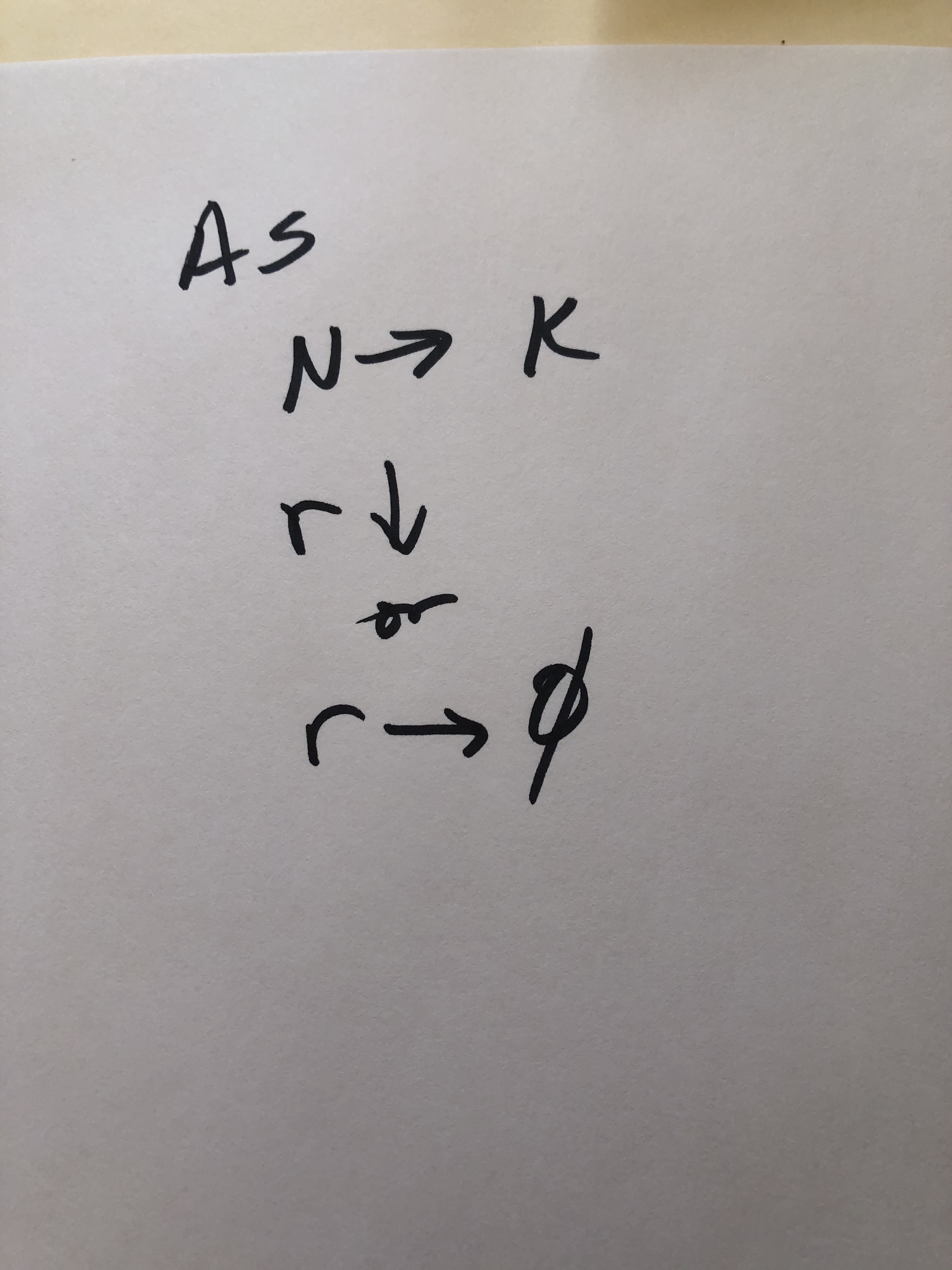
I asked, “When N approaches K, when N = 1000, what do we know about “r”. How much will the population be changing if the graph is level? They answered back that the population isn’t growing at all so “r” must be 0 at that point. What can we multiply times “r” to get 0? They answered zero with an eye roll thrown in for good measure. Interestingly, it wasn’t so easy early in the growth graph to explain what “r” was doing. Since the s-shaped graph starts off slowly the students had a hard time realizing that “r” would be at its maximum value. But after a bit of discussion, they came to that conclusion. Now, I had to get them to understand that the expression is still there. What should the expression evaluate so that when it is multiplied times “r”, “r” will remain at its maximum value? Finally, they came up with 1. I also took the time to work the equation with actual numbers instead of symbol variables at both ends of the curve–so that they were able to see small “N” values and “K” values and what was changing. Now they had something to work with and they went back to their computers.
When you and your students work so hard for something it can be a bit unnerving to face the possibility of failure–that all this effort was wasted. I could have told them the logistic two days ago. I’m sure that most resented that we were working on such a “meaningless idea”. But like I said, I can be a bit stubborn and I was confident that they “could” figure it out but “would” they? They had trusted me to this point but I was losing them.
Suddenly, one of my female students jumped 2 feet in the air and shouted: “I’ve got it!” It is a special day when a student gets so excited about something in the classroom and without that struggle, she wouldn’t have felt such success. I looked over and sure enough, she had this beautiful S-shaped curve. I told her to quickly shut off her monitor (but not her computer) so that others couldn’t see her equation. I wanted everyone to experience her joy. It was pretty amazing. Within the next 15 minutes, the entire class finally had the s-curve. No doubt, some provided a bit of extra help to their neighbors but it was a great day. One, that I had a lot of doubts about going in. The google sheet link reference above has the logistic model as the third tab. The energy went way up in the room and they wanted a bit more. We started out by testing/stressing this model–what happens when you change “r” values? How do you do that systematically? How would this work in a real population?
I imagine you are wondering at this point what the students turned in to be graded. Actually, I don’t remember if they turned anything in. I had witnessed how each struggled through building their spreadsheet models. I had observed the graphs on each screen. I know I had them record their graphs, equations, and notes in their lab notebooks but I imagine that was it. I was more excited about how obviously valued the experience was for almost all students. I wanted them to learn about mathematical models and populations–something that is notoriously difficult to study in a high school classroom but computer access changed that. Or at least in my classes, it did.
The funny thing is, I should have been satisfied with what we accomplished but I figured I’d chance it just a bit more. To see if the students could take on one more challenge. That is the topic of the next post.